Pitch Plotter service allows a user to get graphical image of the pitch frequency contour of a speech phrase online. A phrase audio phonogram of the length no more than a minute is given to the input of the service. The audio phonogram can be uploaded to the service from a hard disk drive of the computer or by an Internet reference, the phonogram must be in .wav format or recorded via service audiorecording options. At the output are the oscillograms, spectrograms and patterns of main pitch contour of the downloaded phrase.
Main terms and concepts
The pitch frequency (PF) is one of the most important physical parameters of the speech signal. From the acoustics viewpoint, it is a first harmonic tonal signal component , which usually carries the maximum energy. The presence of the pitch frequency is a specific feature for vocalized sounds (all vowels and some of consonants, for example, voiced consonants), and vice versa, its absence is indicative for voiceless consonants. PF contour dynamics has a direct correlation with the prosodic features of speech, such as:
- Melodics (PF motion)
- Rhythmic (current change of sounds and pauses length)
- Energy (current change in sound intensity)
Practical value
Exact identification and analysis of these parameters are very important steps in speech research of different specialists (phoneticians, audio experts etc.), in order to determine various prosodic and intonation occurrences of oral speech. The service can be used in programs for foreign languages intonation study, applications of phonoscopy expert determination.
Particular qualities of the service
The service uses a percept algorithm for PF calculating which is named SWIPE [1], this algorithm is based on human auditory perception model. The algorithm is one of the highest quality and most common algorithms for PF determining today [2].
User interface description
The graphic interface of the service includes following basic parts shown in Figure 1.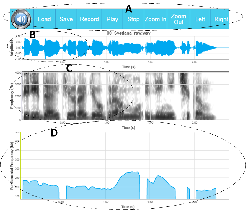
Figure 1. Graphical interface of the service
Command Menu (A) contains the following items:
- Load – to upload the audio file from the computer local disk or other location via URL (the audio file must be in WAV format).
- Save – to save an audio file (or its fragment) on the user’s local disk.
- Record – to start microphone recording, if it is available and connected to user’s computer.
- Play –to listen to an audio file or a part of it (depending on whether an entire file or only a fragment of it is currently displayed and processed in the oscillogram window. Details of the work with a fragment will be described hereinafter).
- Stop – to stop an audio file listening.
- Zoom In – to expand the fragment of the file, marked by left and and right borders markers. Left border marker is indicated by green colour and can be set by clicking the left mouse button in the oscillogram window. Right border marker is indicated by red colour and can be set by clicking the right mouse button in the oscillogram window. More detailed description will be given hereinafter.
- Zoom Out – to reduce the fragment of the file, return to the overview of an entire file.
- Left – to shift the file on one window to the left.
- Right – to shift the file on one window to the right.
- Oscillogram of the signal (B) – a two-dimensional temporal signal reflection. More precisely, it is a dependence of the signal amplitude on the time: abscissas axis (x) – time, ordinates axis (y) – signal amplitude. This graph clearly shows the signal energy dynamics and changes in the power of all its components together (tonal, noise).
- Signal spectrogram (C) – a three-dimensional time-and-frequency signal reflection. More specifically, it is a signal power dependence on the time and frequency simultaneously: abscissas axis (x) – time, ordinate axis (y) – frequency, applicate axis (z) – signal strength (in this case, instead of using a separate axis the color is used: the greater color intensity, the greater is a power signal at this frequency at a given time). In contrast to the oscillogram, spectrogram allows to see separate input of signal components, which have maximum energy at a particular time (tonal or noise components, harmonics in particular, etc.).
- Pitch contour frequency graph (D) – a two-dimensional view of PF value evolution depending on time. Abscissas axis (x) – time, ordinate axis (y) – frequency (Hz). The absence means unvoiced utterance (e.g., voiceless consonants k, ch, č, š, t, s, f ).
User scenarios of working with the service
Scenario 1: Displaying the PF contour of an audio file stored on the local computer’s drive
1.1 To open the service page.
1.2 To press the Load button.
1.3-a To click “Choose File” in a file selection window. The standard operating system dialogue window will be opened for selecting a file on a disk. To select a file from the local disk.
1.3-b To enter the URL of the file that is on the network in the window, for example, http://corpus.by/tts3/cache/out/2015-11-26_21-39-53_134-17-130-18_931_bel_ssrlab.wav
1.4 To wait for oscillogram displaying, spectrogram and PF contour calculation (Figure 2).

Figure 2. Oscillogram, spectrogram and PF contour displaying
Scenario 2: Displaying the PF contour of an audio recorded file with the microphone
2.1 To ensure that your microphone is connected and working.
2.2 To open the service page “Pitch Plotter”.
2.3 To press the Record button.
2.4 To accept browser’s offer to start recording.
2.5 To record a phrase or several phrases, watching the final signal in the oscillogram window in real time.
2.6 To press stop button to stop recording and displaying the results.
2.7 If it is necessary to save the phrase on the computer, to press the Save button.
Scenario 3: Work with a part of an audio file
3.1 To do all the steps of Scenario 1 or Scenario 2, at the user’s choice.
3.2 To put fragment’s left border marker. To do this, move the mouse over any of the area of fragment and press the left button. Green line should appear – it is the left border fragment (Figure 3).
3.3 To put fragment’s right border marker. To do this, move the mouse over any of the area of fragment to the right of the left boundary and press the right button. Red line should appear – it is the right border fragment (Figure 3).

Figure 3. Markers of the fragment’s left and right borders
3.4 To press the Zoom In button to enlarge the marked signal fragment (Figure 4).

Figure 4. Enlarged fragment
3.5 In this mode it is possible to use functions of vocalisation and saving of an audio signal in the context of a given fragment. This means that only chosen signal fragment will be played and saved.
3.6 If it is necessary to zoom in, you should repeat steps 3.2-3.5.
3.7 To return back to the previous scale – press Zoom Out.
3.8 In the mode of the Zoom, when you press Left and Right buttons, there is a shift of the current track signal on one track (one screen) to the left, or one track (one screen) to the right side along the time axis.
Model, algorithm
From the mathematical viewpoint the information processing in the service “Pitch Plotter” can be introduced with the help of the following expression:
\[\left(\ \textbf{o,S,p}\ \ \right)={\mathcal P}\left(\textbf{x}\right),\]
where $\textbf{x}=\left\{x\left(n\right)\ |\ x\in R,\ n=\overline{0,1,2,\dots ,N-1}\right\}\ $ – counting vector of an input speech signal. The signal was received from wav-file, which had been downloaded with the help of the “Load” command, or recorded from the user’s microphone with the help of the “Record” command, $n$ – counting number in the signal;
where $\textbf{o}=\left\{o\left(n\right)\ |\ o\in R,\ n=\overline{0,1,2,\dots ,N-1}\right\}\ $ – signal oscillogram (vector of plot points values on the oscillogram), $n$ – counting number in the signal;
where $\textbf{S}=\left\{s\left(k,m\right)\ |\ s\in R,\ m=\overline{0,1,2,\dots ,M-1},\ k=\overline{0,1,2,\dots ,K-1}\ \right\} $ – signal spectrogram (matrix of plot points values on the spectrogram), $k$ – number of signal harmonic, $m$ – number of signal frame;
where $\textbf{p}=\left\{p\left(m\right)\ |\ p\in R,\ m=\overline{0,1,2,\dots ,M-1}\right\} $ – frequency pitch plot (vector of plot points values), $m$ – number of signal frame.
Therefore, it can be affirmed that ${\mathcal P}$ function, which describes work of the service, consists of superposition of three generations:
\[\left\{ \begin{array}{c}
\textbf{x}\ {{\stackrel{{{\mathcal P}}_o}{\longrightarrow}\ \textbf{o}}}, \\
\textbf{x}\ {{\stackrel{{{\mathcal P}}_s}{\longrightarrow}\ \textbf{S}}}, \\
\textbf{(x,S)}\ {{\stackrel{{{\mathcal P}}_{x,S}}{\longrightarrow}\ \textbf{p}}} \end{array}
\right\}\]
Let’s look each of them in more detail:
- To receive signal oscillogram, there is no need in execution any generations of input data, received counting can be displayed at once. Therefore, ${{\mathcal P}}_o$ function looks like:
\[\textbf{o}={{\mathcal P}}_o\left(\textbf{x}\right)\Longrightarrow \textbf{o}\left(n\right)=1\cdot x\left(n\right)\Longrightarrow \textbf{o}\Longleftrightarrow \textbf{x}.\]
- To receive ${{\mathcal P}}_s$ and ${{\mathcal P}}_p$ discrete Fourier transform (DFT) is used, which we look in more detail. DFT allows to transfer from time to frequency domains, where separate signal components (harmonics) are better seen and its analysis can be made easier (figure 5.1).

Figure 5.1. Transfer from time to frequency domains
Let’s write formula of Fourier transform:
\[X\left(f\right)={\mathcal F}\left(x\left(t\right)\right)=\int^{+\infty \ }_{-\infty \ }{x\left(t\right)\cdot e^{-jwt}dt,} \\ – \infty < t <+\infty,- \infty< f <+ \infty\ \]
Let’s go to the discrete form of transformation, executing the time and frequency values extent discretization/sampling:
\[t=n\cdot T_s,\ ~n=\overline{0,1,\dots ,N-1}\ \]
\[f=k\cdot F_1,\ ~k=\overline{0,1,\dots ,K-1}\]
where $T_s$ – signal discretization period, $F_1$ – frequency of the first signal harmonic. Then, Fourier transform in the discrete form will be:
\[X[k]={\mathcal F}\left(x[n]\right)=\sum^N_{n=1}{x[n]\cdot e^{-j2\pi (k\cdot F_1)(n\cdot T_s)}}\]
This expression can be introduced in matrix form as:

Figure 5.2. Fourier transform in matrix form
As Fourier transform kernel $e^{-jwt}$ has a complex form, then to gain a better understanding of physical meaning let’s write down harmonic functions in real form with the help of Euler transformation, which has the following form:
\[e^{-j\varphi }=cos\varphi -jsin\varphi \]
\[X[k]={\mathcal F}\left(x[n]\right)=\sum^N_{n=1}{x[n]\cdot (cos(2\pi kF_1nT_s)-jsin(2\pi kF_1nT_s))}\]

Figure 5.3. Harmonic functions in a real form, written down with the help of Euler transformation
To receive a spectrogram, Fourier transform is executed for each $m$–frame of $r$-signal:
$r$-frame – is a signal segment with a length of $L$ counting, which is named frame in signal processing.
\[r_m=\{x\left[l\right],\ ~l=\overline{m\cdot t,m\cdot t+1\dots m\cdot t+L}\ ,\ m=\overline{0,\ \dots ,M}\ \ \},\]
where $l$ – number of signal counting in the interior of frame, $m$ – frame number, $t$ – step of signal analysis, $L$ – frame elongation in counting.
Therefore, ${{\mathcal P}}_S$ function looks like:
\[\textbf{S}={{\mathcal P}}_S\left(\textbf{x}\right)\Longrightarrow S=abs({\mathcal F}(x\left[k,m\right])).\]
- To receive the contour of pitch it is necessary to use SWIPE estimator (a sawtooth waveform inspired pitch estimator). It uses time and frequency signal notation. Procedure, which executes this algorithm, is fairly complicated, and then will not be considered here. For those, who is interested in it is possible to find the specified mathematical description by the reference [1].
Therefore, ${{\mathcal P}}_{o,S}$ function looks like:
\[\textbf{p}={{\mathcal P}}_{o,S}\left(\textbf{x,S}\right)=SWIPE(\textbf{x,S}).\]
And therefore, we considered the mathematical model of the service Pitch Plotter.
Source references
Video tutorial for work with this service: Pitch Plotter tutorial – Corpus.by
Service page: http://corpus.by/PitchPlotter/?lang=be
Cross-references
- SWIPE
- Instantaneous Pitch Estimation based on Rapt Framework
- Русак, В.П. Программная обработка фонетических особенностей белорусских говоров центрального региона / В.П. Русак, Ю.С. Гецевич // Исследования по славянской диалектологии 19–20. Славянские диалекты в современной языковой ситуации. Диалектный словарь как способ исследования славянских диалектов / отв. редактор выпуска: д. ф. н. Л. Э. Калнынь. — Москва : Институт славяноведения РАН, 2018. — C. 87-94.